Shot charts
blazing-the-nets draws a team's or a player's shots three ways: hexagons on the court
coloured by FG% against the league and sized by attempts, the court's zones filled the same way, and a shooting
signature of FG% by distance. Its current app (main, Next.js) and its 2021 one (master, React and d3) compute
these differently. @sportsdataverse/sdvplot/shots computes both, main's by default and master's through
options. It imports neither Plot nor d3, so it runs on a server or in a worker. @sportsdataverse/sdvplot/plot and
@sportsdataverse/sdvplot/d3 draw what it computes.
The data
The input is rows of the sportsdataverse-data nba_stats_shots release: x_legacy and y_legacy in tenths of a
foot from the hoop, shot_distance in feet, shot_value (2 or 3) and shot_result ("Made" or "Missed"). Rows
from stats.nba.com's shotchartdetail, which master read, take one .map: LOC_X and LOC_Y become x_legacy
and y_legacy, SHOT_DISTANCE becomes shot_distance, a SHOT_MADE_FLAG of 1 becomes "Made" (anything else
"Missed"), and a SHOT_TYPE of "3PT Field Goal" becomes a shot_value of 3 (anything else 2). Only the zones read
shot_value. The examples on this page draw Brooklyn's first 2000 shots of 2025-26 against that season's league (see
Sample data).
[
  {
    "x": 0,
    "y": 0,
    "attempts": 2,
    "makes": 1,
    "fgPct": 0.5,
    "meanDistance": 0.5,
    "zone": "restricted_area"
  },
  {
    "x": -45,
    "y": 255,
    "attempts": 1,
    "makes": 1,
    "fgPct": 1,
    "meanDistance": 26,
    "zone": "above_break_3"
  }
]
import { binShots } from "@sportsdataverse/sdvplot/shots";
const shots = [
{ x_legacy: -1, y_legacy: 7, shot_distance: 1, shot_value: 2, shot_result: "Made" },
{ x_legacy: 0, y_legacy: 0, shot_distance: 0, shot_value: 2, shot_result: "Missed" },
{ x_legacy: -44, y_legacy: 252, shot_distance: 26, shot_value: 3, shot_result: "Made" },
];
binShots(shots, 15);
binShots(shots, { shape: "square", side: 15 });
A hex chart against the league
Each cell carries two numbers: its colour is the FG% there minus the league's, and its size is the attempts.
cellsVsLeague compares each cell with the league in the same cell, from a leagueIndex of the whole season; a cell
the league shot fewer than 25 times from takes its zone's league rate. master compared each cell with the league's
FG% at the cell's distance instead (cellsVsDistance), drew 1 ft cells, sized them linearly up to a cap and coloured
the raw difference. main shrinks the difference toward the league by 25 attempts, so a 2-for-2 cell does not read as
the hottest spot on the floor.
import * as Plot from "@observablehq/plot";
import { BKN_SHOTS_2026, NBA_LEAGUE_2026 } from "@sportsdataverse/examples/data";
import { shotCells, surface } from "@sportsdataverse/sdvplot/plot";
import { cellsVsDistance, cellsVsLeague, diffScale, sizeCells } from "@sportsdataverse/sdvplot/shots";

// Brooklyn's first 2000 shots of 2025-26 against the 2025-26 league, hoop at the bottom. Colour is a cell's FG% minus
// the league's; size is its attempts.
const court = surface("nba", { displayRange: "defense", rotation: 90 });
const frame = "nba-legacy-vertical";

// main: 1.5 ft hexagons against the league in the same hexagon, shrunk toward it by 25 attempts, sized by "sqrt-p95"
const main = cellsVsLeague(BKN_SHOTS_2026, NBA_LEAGUE_2026.hex15);
const mainSizes = sizeCells(main, NBA_LEAGUE_2026.hex15);
// master: 1 ft hexagons against the league at the hexagon's distance, the raw difference, sized by "linear-cap"
const master = cellsVsDistance(BKN_SHOTS_2026, NBA_LEAGUE_2026.byFoot, 10);
const masterSizes = sizeCells(master, { radius: 10, rule: "linear-cap" });
const masterScale = diffScale({ palette: "master" });

// diffScale's domain is a fraction (0.15 is 15 points): label the ticks in points, as d3's appendLegend does
const pts = (d: number): string => (d === 0 ? "0" : `${d > 0 ? "+" : "−"}${Math.abs(d * 100).toFixed(1)}`);

const panel = (caption: string, cells: Plot.Markish, scale: ReturnType<typeof diffScale>): HTMLDivElement => {
  const div = document.createElement("div");
  div.append(
    Plot.plot({ ...court.scales, width: 420, caption, marks: [...court.marks, cells] }),
    Plot.legend({ color: { ...scale.plot, label: "FG% vs league (points)", tickFormat: pts } }),
  );
  return div;
};

const charts = document.createElement("div");
charts.style.cssText = "display: flex; flex-wrap: wrap; gap: 16px";
charts.append(
  panel(
    "main: 1.5 ft hexagons against the league in the same hexagon",
    shotCells(main, { r: mainSizes.r, frame, tip: true }),
    diffScale(),
  ),
  panel(
    "master: 1 ft hexagons against the league at the same distance",
    shotCells(master, { r: masterSizes.r, prior: 0, scale: masterScale, frame, tip: true }),
    masterScale,
  ),
);
charts;
0.07937540663630449
import { LEAGUE_PRIOR_ATTEMPTS, shrunkDiff } from "@sportsdataverse/sdvplot/shots";

shrunkDiff(4, 4, 270 / 636, LEAGUE_PRIOR_ATTEMPTS); // +0.08, not the raw +0.58
shotCells draws the cells as Plot.geo through the plot's own scales, so a cell is exact in court feet. The
nba-legacy-vertical frame puts the hoop at the bottom of a court drawn with rotation: 90.
Hexagons or squares
Both shapes bin the same shots into cells with the same counts, colours and sizes; only the outline differs. A
hexagon's six neighbours all sit at the same distance from its centre, and its corners stay close to that centre, so a
hot spot spreads evenly and the lattice adds little direction of its own to the picture. That is why both
blazing-the-nets apps use hexagons. Squares line up with the court's straight lines (the lane, the baseline, the
corner-three strips) and read as a grid, so a cell is easy to name and to compare along a row or column. Their corners
reach farther from the centre (s/√2 against r), so a square groups slightly less local shots than a hexagon of the
same area. For a like-for-like comparison, give the squares the hexagon's area:
{ shape: "square", radius: 10, equalArea: true } makes squares of side 16.12 tenths of a foot, 378 of them for these
2000 shots against 374 hexagons of radius 10. The league context for those squares is
NBA_LEAGUE_SQUARE_2026, the same season's shots binned by sdvplot's own squarebin.
import * as Plot from "@observablehq/plot";
import { BKN_SHOTS_2026, NBA_LEAGUE_2026, NBA_LEAGUE_SQUARE_2026 } from "@sportsdataverse/examples/data";
import { shotCells, surface } from "@sportsdataverse/sdvplot/plot";
import { type LeagueIndex, cellsVsLeague, sizeCells } from "@sportsdataverse/sdvplot/shots";

// Brooklyn's first 2000 shots of 2025-26 against the 2025-26 league twice: in 1 ft hexagons (radius 10), and in
// squares of the same area (side 16.1 tenths of a foot). Each league index bins the league on its own lattice and
// the player is binned on the index's lattice, so only the cell outline differs.
const court = surface("nba", { displayRange: "defense", rotation: 90 });
const panel = (name: string, index: LeagueIndex, shape: "hex" | "square"): SVGSVGElement | HTMLElement => {
  const cells = cellsVsLeague(BKN_SHOTS_2026, index);
  return Plot.plot({
    ...court.scales,
    width: 420,
    caption: `${name}: ${cells.length} cells`,
    marks: [
      ...court.marks,
      shotCells(cells, { r: sizeCells(cells, index).r, shape, frame: "nba-legacy-vertical" }),
    ],
  });
};

const charts = document.createElement("div");
charts.style.cssText = "display: flex; flex-wrap: wrap; gap: 16px";
charts.append(
  panel("Hexagons, radius 10", NBA_LEAGUE_2026.hex10, "hex"),
  panel("Squares of the same area", NBA_LEAGUE_SQUARE_2026, "square"),
);
charts;
sdvplot/bins holds the binners alone, without sporty: binner, hexbin and squarebin take any points and x/y
accessors, and binner(...).cell(px), hexagonPath and squarePath give the outline to draw at each centre.
import { BKN_SHOTS_2026 } from "@sportsdataverse/examples/data";
import { type BinOf, binner, squarePath, squarebin } from "@sportsdataverse/sdvplot/bins";
import * as d3 from "d3";

// sdvplot/bins knows nothing of basketball (it does not import sporty): give it points and x/y accessors. Here,
// Brooklyn's first 2000 shots of 2025-26 in tenths of a foot from the hoop, binned once by binner into hexagons of
// radius 15 and once by squarebin into squares of side 15, and drawn the d3-hexbin way: one path per cell,
// translated to its centre and shaded by its count.
type Shot = (typeof BKN_SHOTS_2026)[number];
const shots = BKN_SHOTS_2026.filter((s) => s.y_legacy <= 420);
const k = 0.6; // px per tenth of a foot
const [w, h] = [500 * k, 470 * k];
const x = d3.scaleLinear([-250, 250], [0, w]);
const y = d3.scaleLinear([-50, 420], [h, 0]);
const hex = binner({ radius: 15 });
const panels: { title: string; bins: BinOf<Shot>[]; path: string }[] = [
  {
    title: "binner({ radius: 15 })",
    bins: hex.bins(shots, { x: (s) => s.x_legacy, y: (s) => s.y_legacy }),
    path: hex.cell(15 * k),
  },
  {
    title: "squarebin(…, { side: 15 })",
    bins: squarebin(shots, { side: 15, x: (s) => s.x_legacy, y: (s) => s.y_legacy }),
    path: squarePath(15 * k),
  },
];

const most = d3.max(panels, (p) => d3.max(p.bins, (b) => b.length)) ?? 1;
const shade = d3.scaleSequentialLog(d3.interpolateBlues).domain([1, most]);
const svg = d3
  .create("svg")
  .attr("viewBox", [0, 0, 2 * w + 20, h + 24])
  .attr("width", 2 * w + 20);
panels.forEach((p, i) => {
  const g = svg.append("g").attr("transform", `translate(${i * (w + 20)},24)`);
  g.append("rect")
    .attr("width", w)
    .attr("height", h)
    .attr("fill", "none")
    .attr("stroke", "currentColor")
    .attr("stroke-opacity", 0.3);
  g.append("text")
    .attr("y", -8)
    .attr("font-size", 12)
    .attr("fill", "currentColor")
    .text(`${p.title}: ${p.bins.length} cells`);
  g.selectAll("path")
    .data(p.bins)
    .join("path")
    .attr("d", p.path)
    .attr("transform", (b) => `translate(${x(b.x)},${y(b.y)})`)
    .attr("fill", (b) => shade(b.length))
    .attr("stroke", "white")
    .attr("stroke-width", 0.3);
});
svg.node();
Zones
statsByZone counts makes and attempts in the six zones (restricted area, paint, mid-range, both corner threes,
above the break). shotZones fills sporty's basketballZones with a colour per zone and labels each one, here
makes/attempts. Build the zones with scale: 10 so they are in the shots' tenths, and pass the shots' frame.
import * as Plot from "@observablehq/plot";
import { BKN_SHOTS_2026, NBA_LEAGUE_2026 } from "@sportsdataverse/examples/data";
import { shotZones, surface } from "@sportsdataverse/sdvplot/plot";
import { diffScale, shrunkDiff, statsByZone } from "@sportsdataverse/sdvplot/shots";
import { type BasketballZone, basketballZones } from "@sportsdataverse/sporty";

// Brooklyn's first 2000 shots of 2025-26 by zone, each zone filled by its FG% minus the 2025-26 league's in that
// zone, shrunk toward the league by 25 attempts, and labelled makes/attempts.
const player = statsByZone(BKN_SHOTS_2026);
const league = NBA_LEAGUE_2026.hex15.zones;
const colour = diffScale();
const diff = (z: BasketballZone): number | null => {
  const rate = league[z].fgPct;
  return rate === null ? null : shrunkDiff(player[z].makes, player[z].attempts, rate);
};

// The zones are built in legacy tenths (scale: 10), so they take the shots' frame to land on this court.
const court = surface("nba", { displayRange: "defense", rotation: 90 });
Plot.plot({
  ...court.scales,
  width: 500,
  marks: [
    ...court.marks,
    ...shotZones(basketballZones("nba", { scale: 10, top: 350 }), {
      fill: (z) => colour(diff(z)),
      text: (z) => `${player[z].makes}/${player[z].attempts}`,
      frame: "nba-legacy-vertical",
      stats: player,
      tip: true,
    }),
  ],
});
Shooting signature
signaturePoints turns FG% by distance against the league into a ribbon: its height is the FG%, its width the share of
shots taken from there, and its colour the shrunk difference from the league, whose FG% is the dashed line.
shootingSignature draws it in Plot; appendSignature in d3.
import * as Plot from "@observablehq/plot";
import { BKN_SHOTS_2026, NBA_LEAGUE_2026 } from "@sportsdataverse/examples/data";
import { shootingSignature } from "@sportsdataverse/sdvplot/plot";
import { diffScale, fgPctByDistance, signaturePoints, vsLeague } from "@sportsdataverse/sdvplot/shots";

// FG% by distance for Brooklyn's first 2000 shots of 2025-26, as wide as the share of shots taken from there and
// coloured by FG% minus the 2025-26 league's (the dashed line), shrunk toward the league by 25 attempts.
const points = signaturePoints(vsLeague(fgPctByDistance(BKN_SHOTS_2026), NBA_LEAGUE_2026.byFoot));
// diffScale's domain is a fraction (0.15 is 15 points): label the ticks in points, as d3's appendLegend does
const pts = (d: number): string => (d === 0 ? "0" : `${d > 0 ? "+" : "−"}${Math.abs(d * 100).toFixed(1)}`);

const figure = document.createElement("div");
figure.append(
  Plot.plot({
    width: 640,
    x: { label: "Distance (ft)" },
    y: { domain: [0, 1], label: "FG%", tickFormat: "%" },
    marks: shootingSignature(points, { tip: true }),
  }),
  Plot.legend({ color: { ...diffScale().plot, label: "FG% vs league (points)", tickFormat: pts } }),
);
figure;
Hover
The three Plot marks take tip: true, as the hex chart, zones and signature above do: hover them. A cell shows its
attempts, FG%, the league's FG% and the shrunk difference; a zone shows its name and, when shotZones is given
stats (statsByZone(shots)), its makes/attempts and FG%; the signature shows the distance, FG%, the league's FG%
and the share of shots where the pointer is. A tip object's format overrides sdvplot's formats key by key.
shotZones and shootingSignature return the tip as their last mark, so spread them last, or add other marks before
them: a mark added after them paints over the tip.
shotCells' dropOutside (default true) leaves out cells whose centre is outside the frame, so a tip never points
at a cell that is not drawn; Plot's own clip passes through and cuts paths at the frame instead.
Linking
Each cell's path carries data-sdv-id, the cell's legacy centre as "x,y", and each zone's carries the zone's name,
so @sportsdataverse/sdvplot/interact links the charts with no glue code.
linkSelection(store, { figure, select: "toggle" }) makes every hexagon (or zone) a checkbox: a click, Enter or Space
toggles its id in the store's selected, and the other cells dim. Its hover: { id: (h) => `${h.x},${h.y}` }
writes the cell Plot's tip points at, the nearest within tip: { maxRadius: 18 }, as main does. linkCursor
follows one shot distance: on the court a ring around the hoop (shape: { axis: "ring", center: [0, -41.75] } in the
vertical frame), on the signature a rule, and the signature writes the distance under the pointer. Hexagon ids and
zone names are two id spaces, so each gets its own store; on one store a hovered hexagon would dim every zone. A click
also pins Plot's tip, so give it pointerEvents: "none" (tip: { maxRadius: 18, pointerEvents: "none" }): the pinned
tip then never takes a click meant for a hexagon under it, and its hexagon stays hovered until the next click on the
court. Squares link the same way.
import * as Plot from "@observablehq/plot";
import { BKN_SHOTS_2026, NBA_LEAGUE_2026 } from "@sportsdataverse/examples/data";
import { createSelection } from "@sportsdataverse/sdvplot";
import { linkCursor, linkSelection } from "@sportsdataverse/sdvplot/interact";
import { shootingSignature, shotCells, shotZones, surface } from "@sportsdataverse/sdvplot/plot";
import {
  type CellVsLeague,
  cellsVsLeague,
  diffScale,
  fgPctByDistance,
  shrunkDiff,
  signaturePoints,
  sizeCells,
  statsByZone,
  vsLeague,
} from "@sportsdataverse/sdvplot/shots";
import { BASKETBALL_ZONE_LABELS, basketballZones } from "@sportsdataverse/sporty";

// Brooklyn's first 2000 shots of 2025-26 against the 2025-26 league, hoop at the bottom. Click a hexagon or a zone to
// select it (or Tab to it and press Enter or Space); hover the court for the nearest hexagon within 18 px; hover the
// signature and the court rings that distance around the hoop.
const D = "shot_distance";
const frame = "nba-legacy-vertical";
const pct = (v: number | null): string => (v === null ? "n/a" : `${(v * 100).toFixed(1)}%`);
const pts = (v: number): string => `${v >= 0 ? "+" : "−"}${Math.abs(v * 100).toFixed(1)}`;
// Hexagon ids ("x,y") and zone names are two id spaces, so each gets its own store: on one store a hovered hexagon
// would dim every zone.
const store = createSelection();
const zoneStore = createSelection();

// blazing-the-nets main's chart: 1.5 ft hexagons against the league in the same hexagon, its four tip lines
const cells = cellsVsLeague(BKN_SHOTS_2026, NBA_LEAGUE_2026.hex15);
const court = surface("nba", { displayRange: "defense", rotation: 90 });
const hexes = Plot.plot({
  ...court.scales,
  width: 500,
  marks: [
    ...court.marks,
    shotCells(cells, {
      r: sizeCells(cells, NBA_LEAGUE_2026.hex15).r,
      frame,
      tip: { maxRadius: 18, pointerEvents: "none" }, // a pinned tip lets a click through to the hexagon under it
      title: (h: CellVsLeague) =>
        [
          BASKETBALL_ZONE_LABELS[h.zone],
          `${h.makes}/${h.attempts} FG, ${pct(h.fgPct)}`,
          `League ${pct(h.leagueFgPct)}${h.fgPct !== null && h.leagueFgPct !== null ? ` (${pts(h.fgPct - h.leagueFgPct)})` : ""}`,
          `${h.meanDistance.toFixed(1)} ft`,
        ].join("\n"),
    }),
  ],
});
linkSelection(store, {
  figure: hexes,
  select: "toggle",
  hover: { id: (h: CellVsLeague) => `${h.x},${h.y}` },
});
linkCursor(hexes, store, {
  field: D,
  shape: { axis: "ring", x: hexes.scale("x")!, y: hexes.scale("y")!, center: [0, -41.75] }, // the vertical frame's hoop
});

// The zones, each filled by its FG% against the league's in that zone and labelled makes/attempts
const player = statsByZone(BKN_SHOTS_2026);
const colour = diffScale();
const zones = Plot.plot({
  ...court.scales,
  width: 500,
  marks: [
    ...court.marks,
    ...shotZones(basketballZones("nba", { scale: 10 }), {
      fill: (z) => {
        const rate = NBA_LEAGUE_2026.hex15.zones[z].fgPct;
        return colour(rate === null ? null : shrunkDiff(player[z].makes, player[z].attempts, rate));
      },
      text: (z) => `${player[z].makes}/${player[z].attempts}`,
      frame,
    }),
  ],
});
linkSelection(zoneStore, { figure: zones, select: "toggle" });

// The shooting signature writes the distance under the pointer, one value per foot
const signature = Plot.plot({
  width: 500,
  height: 220,
  x: { label: "Shot distance (ft)" },
  y: { domain: [0, 1], label: "FG%", tickFormat: "%" },
  marks: shootingSignature(
    signaturePoints(vsLeague(fgPctByDistance(BKN_SHOTS_2026), NBA_LEAGUE_2026.byFoot)),
    { curve: "basis" },
  ),
});
linkCursor(signature, store, {
  field: D,
  shape: { axis: "x", scale: signature.scale("x")! },
  snap: (feet) => Math.floor(feet) + 0.5,
});

store.set({ cursor: { field: D, value: 26.5 } }); // just behind the arc: Brooklyn's busiest foot
const root = document.createElement("div");
root.style.cssText = "display: flex; flex-wrap: wrap; gap: 16px; align-items: flex-start";
root.append(hexes, zones, signature);
root;
The linked shot dashboard adds master's bar and side charts on the same distance.
Legends
The colours come from diffScale(), a function from a difference to a colour. Its .plot is the same scale in
Observable Plot's terms, so Plot.legend({ color: diffScale().plot }) draws the matching colour bar, as the charts
above do; they pass a tickFormat so its ticks read in percentage points, as appendLegend's do. In d3, appendLegend draws the bar, a caption and, given sizeCells' sizes, a key of cell sizes.
import { BKN_SHOTS_2026, NBA_LEAGUE_2026 } from "@sportsdataverse/examples/data";
import { appendLegend } from "@sportsdataverse/sdvplot/d3";
import { LEAGUE_PRIOR_ATTEMPTS, cellsVsLeague, diffScale, sizeCells } from "@sportsdataverse/sdvplot/shots";
import { create } from "d3";

// The key of blazing-the-nets main's hex chart: the colour bar of diffScale(), then a size key whose steps are 1,
// half the cap and the cap, for Brooklyn's 2025-26 shots in 1.5 ft hexagons. Sizes are in tenths of a foot, drawn
// here at one pixel per tenth.
const cells = cellsVsLeague(BKN_SHOTS_2026, NBA_LEAGUE_2026.hex15);
const sizes = sizeCells(cells, NBA_LEAGUE_2026.hex15);
const svg = create("svg").attr("viewBox", "0 0 300 200").attr("width", 300);
const height = appendLegend(svg.append("g"), diffScale(), {
  width: 280,
  notes: [`FG% is shrunk toward the league's by ${LEAGUE_PRIOR_ATTEMPTS} attempts.`],
  size: { px: sizes.size, steps: sizes.steps },
});
svg.attr("viewBox", `0 0 300 ${height}`);
svg.node();
Faces and initials
appendHeadshots with clip: "circle" crops each headshot to a circle, with an optional ring and a placeholder disc
that stays behind the face if the image does not load.
import { appendHeadshots } from "@sportsdataverse/sdvplot/d3";
import { create } from "d3";

// Seven NFL players by ESPN athlete id, with the names ESPN gives them. clip: "circle" crops each headshot to a face,
// and the placeholder disc stays behind it if the image fails to load.
const players = [
  { id: "4432773", name: "Brian Thomas Jr." },
  { id: "4243389", name: "Calvin Austin III" },
  { id: "4374302", name: "Amon-Ra St. Brown" },
  { id: "4429160", name: "De'Von Achane" },
  { id: "4047646", name: "A.J. Brown" },
  { id: "3133487", name: "Andrew Van Ginkel" },
  { id: "3139477", name: "Patrick Mahomes" },
];
const [width, height] = [700, 120];
const x = (i: number): number => 50 + i * 100;
const svg = create("svg").attr("viewBox", [0, 0, width, height]).attr("width", width);
appendHeadshots(
  svg,
  players.map((_, i) => i),
  players.map(() => 0),
  players.map((p) => p.id),
  {
    league: "nfl",
    x: (v) => x(Number(v)),
    y: () => 50,
    frameHeight: height,
    height: 0.6,
    clip: "circle",
    ring: "#525252",
    placeholder: "#d4d4d4",
  },
);
svg
  .append("g")
  .attr("font-size", 11)
  .attr("text-anchor", "middle")
  .attr("fill", "currentColor")
  .selectAll("text")
  .data(players)
  .join("text")
  .attr("x", (_, i) => x(i))
  .attr("y", 110)
  .text((p) => p.name);
svg.node();
In React, <Headshot fallback="initials" name="…"> shows the player's initials when there is no headshot URL or
the image fails to load, server-rendered pages included.
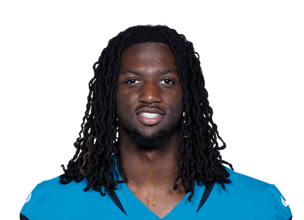 PG
PGimport { Headshot } from "@sportsdataverse/sdvplot/react";
// Brian Thomas Jr. by ESPN athlete id: his headshot. Pete Guerrerio by nflverse gsis id: nflverse's players table
// (players.parquet, 2026-10-08) has no headshot and no ESPN id for him, so there is no URL, and fallback="initials"
// shows "PG" with nothing to download. An image that fails to load falls back the same way.
(
<div style={{ display: "flex", gap: 12, alignItems: "center" }}>
<Headshot playerId="4432773" league="nfl" name="Brian Thomas Jr." fallback="initials" height={80} />
<Headshot
playerId="00-0036454"
league="nfl"
idSystem="gsis"
name="Pete Guerrerio"
fallback="initials"
height={80}
/>
</div>
);
In the gallery: Shot charts, D3 and React.